


Because Psykinematix is a sophisticated tool,
there are usually many ways to solve a given problem. Even when dealing with
an apparently simple stimulus and a powerful computer configuration, we recommend
that, instead of jumping to the most obvious solution, you also consider alternative
solutions. By taking the computational constraints/complexity (eg, the stimulus
structure, its spatial size and duration) into account, you may be able to
minimize the computational requirements of your experiment and make it run
more smoothly. For example, your experimental design may require to create
dynamic stimuli on the fly, or to pre-compute them for every presentation frame,
which would affect both the computation time (and hence appears as a delay
to the user) and the memory usage (both RAM and VRAM). There are several techniques
that can help reduce stimulus memory requirements significantly which is particularly
important for the less powerful configurations.
In this section, you will find a few tips to generate complex stimuli using
various techniques that minimizes these computational requirements. You will
also find more details about some concepts like stereoscopic vision. You
can find demonstrations illustrating most of these techniques in the demos
folder available in the Storage area of the
Designer Panel.
Motion Stimuli
Spatial Aperture
Stereo Stimuli
Using a Cedrus Lumina Controller
How To...?
Let’s consider a typical stimulus used in visual psychophysics, a drifting grating, that needs to be presented with a specific spatial extend and duration. In the past, such a dynamic stimulus would have been created by simply generating a spatial map (in the form of cyclic ramps) and an animated sinusoidal lookup table (LUT). However this technique is now outdated and is not used by Psykinematix because most graphics card are powerful enough to store and compute complex animations. Moreover the OpenGL drivers for Macintosh computers stop supporting this technique across the full range of graphics cards with Mac OS X.
Solution 1: Time-Varying Stimulus
The alternative solution is to create motion
stimuli by generating and storing each frame of the dynamic sequence. In Psykinematix,
this can be done by simply specifying time-varying parameters. For example,
a drifting grating can be made by specifying the value of the spatial phase
parameter as a continuous function of time (assuming a drift of 1 cycle per
second):
where [TIME] is a built-in variable that provides the time of each video
frame (in seconds) relative to the stimulus onset.
Psykinematix will then evaluate the phase parameter and generate a texture
for each video frame. All stimuli parameters in Psykinematix support time-varying
expressions, and very complex stimuli can then be created this way, particularly
when several parameters are simultaneously time-varying.
The use of the [TIME] variable requires the stimulus to be generated as a
texture for every video frame (ie at the display frame rate) for its whole
duration. Though Psykinematix makes sure to not recompute similar frames,
this computation which is performed before the actual presentation may result
in a significant delay if the stimulus duration is too long or the stimulus
too complex. Note that in most cases this stimulus generation should be fast
enough for stimuli that have a short duration (typically less than 1 second).
For longer duration, the use of the [TIME] variable may not be practical.
Fortunately Psykinematix provides other ways to specify time-varying parameters.
If your experiment protocol does not rely on the presentation of temporally
smooth stimuli, there are other time-varying
formats available to specify
values that change at a specified temporal rate that require much less computational
requirements in terms of speed and memory footprint. For example:
to indicate a uniform sampling in the range [min-max] with each sample having
a specified duration. So instead of using the phase expression 360*[TIME] to
create a drifting grating at a speed of 1 cycle per second, one could use the
format:
to create an apparent motion by cycling through 4 spatial phases (0, 90, 180
and 270 deg), this cycle being repeated for the whole duration of the
grating. This could even be combined with a time-varying OpenGL rotation of
180 deg (see rendering options) to create a drifting grating that alternates
in direction at regular intervals (thanks to Alex Wade for this tip!).
Some alternative solutions have to be sought however if a smooth motion
is required and the use of the [TIME] variable is precluded because the
stimulus generation would take too long or require too many textures.
Solution 2: Moving Stimulus!
The most intuitive way to create motion is
actually to simply change the position over time of an otherwise static stimulus.
This is a very fast technique that does not require the recomputation of the
stimulus for each video frame, the stimulus being computed once and then pasted
at a different position for each frame. Though this technique cannot not apply
to any kind of motion stimuli, it looks appropriate for a drifting grating
since a phase shift is equivalent to a spatial shift.
In Psykinematix this can be easily done by specifying time-varying Cartesian
or polar coordinates, for example to move a stimulus horizontally from 5
degrees on the left to 5 degrees on the right in 1 second assuming a constant
speed you would indicate for its x coordinate an expression like:
The problem here is that if the whole grating will move in the visual field
and not appear as simply drifting at a specific location. So this technique
is obviously only appropriate for very simple stimuli (ie very localized
in nature like moving dots).
For more extended stimuli, like a drifting grating, a spatial
aperture (see below) may be required to limit the stimulus presentation
to a static window to create the perception of a drifting stimulus rather than
that of a stimulus moving as a whole. However this would put constraints on
the aperture and stimulus size as well as the drifting speed to prevent the
stimulus from disappearing from the window aperture during the presentation.
An easy fix for this problem that would only work for periodic stimuli is to
reset their position at regular intervals as soon they start to disappear from
the aperture window, using for example the following expression for their
x coordinate (ie motion starting at x = -2 deg to x = 2 deg at a rate of
4 deg/s):
However for non-periodic stimuli, this may not always properly work and the technique would be limited to motion of short durations, but there is a work-around that may work for you as described below.
Solution 3: Sweeping Technique
Rather than using a single stimulus that moves behind the aperture window, a second stimulus could be used to replace the one that leaves the aperture and their roles could be then flipped over as illustrated on the figure below (the 2 sweeps are copies of the same moving stimulus designed so that their border is invisible when put side by side).
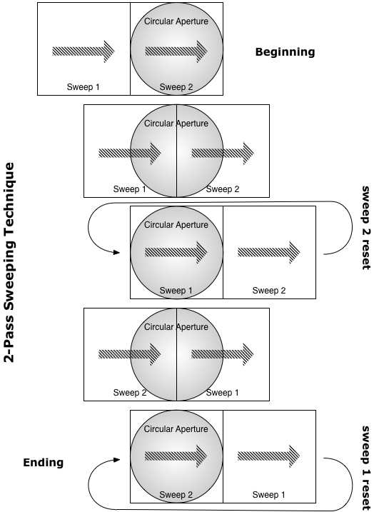
This technique, we call the 2-pass
sweeping technique, can produce motion of infinitely long duration with a minimum of
computational requirements, which is particularly useful for creating adapting
motion stimuli for example (see the 2-Pass Sweeping Technique motion demo in
the Storage area of the Designer Panel). However the difficulty in the implementation
of this technique resides in the proper specification of the time-varying expression
for the position of each sweep: in particular the sweep position needs to be
reset every time one sweep leaves the aperture. Below is an example of such
expression for each sweep and illustrated graphically using Psykinematix Math
palette:
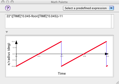
This expression defines the horizontal position
of sweep 1 as starting outside and on the left of the circular aperture (-11
deg), then shifting to the right at a speed of 1 deg/s, before getting reset
to its starting position after 22 seconds (22 deg being the diameter of the
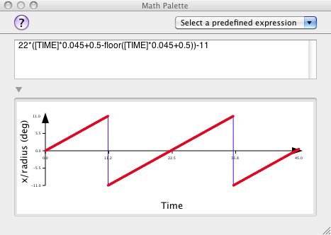
aperture and the size of each sweep stimulus). Similarly the horizontal position
of sweep 2 starts centered on the circular aperture (0 deg), then shifts to
the right at a speed of 1 deg/s, and finally gets reset outside and on the
left of the circular aperture (-11 deg) after 11 seconds:
Though this work-around is probably not obvious to everyone it illustrates how it is possible to reduce the computational requirements to a minimum (2 stimulus textures) using the powerful capabilities found in Psykinematix.
Remember that time-varying expressions for stimulus coordinates (Cartesian & polar) and OpenGL parameters (rotation and scaling, see rendering settings) are applied on the fly and do not require the recomputation of stimulus textures, so try to take advantage of these!
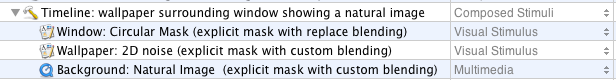
A spatial aperture is a transparent window that let you see only parts of visual stimuli being otherwise hidden by the most front stimuli. The effect is easily computed by multiplying a binary mask (set to 1 for the opaque parts, and 0 for the transparent parts) with the stimulus presented behind the window on a pixel basis. This effect is generally combined with the presentation of another stimulus outside the window (the "wallpaper") as illustrated below and formally described as:
seen result = (1 - mask) x stimulus + mask x wallpaper
result
1 - mask
stimulus
mask
wallpaper
Psykinematix offers several techniques to create a spatial aperture (see the techniques demo in the Storage area of the Designer Panel):
Solution 1: Custom Stimuli
A first solution is to explicitly compute each of the above steps using a
Custom Stimuli as following:
stimulus = f(x,y,r,theta)
mask = g(x,y,r,theta)
wallpaper = h(x,y,r,theta)
z = (1-mask)*stimulus+mask*wallpaper
The main advantage of this technique is that the aperture window and the
stimuli are computed and combined simultaneously with a preview available
of the masked stimulus. This is the recommended technique for beginners.
This technique, however, cannot be used if the stimuli cannot be generated
using mathematical expressions, as it is the case with Multimedia stimuli.
Moreover, if the stimuli are dynamic (time-varying) then the aperture and
the combination are recomputed for every frame that may lead to unneeded
delay.
If the stimulus is already present as the display background, an aperture
can still be created using the za
output component of a custom stimulus and by specifying a 'Transparent' blending mode in its rendering options:
mask = f(x,y,r,theta)
za = mask
A wallpaper can be optionally specified using the z output component:
mask = f(x,y,r,theta)
wallpaper = g(x,y,r,theta)
z = wallpaper
za = mask
Here is an example that would show an image seen through a simple circular aperture which consists in a timeline with a masked stimulus pasted first into video memory, overlapped with a custom mask specified through the za component:
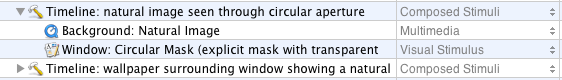
With the 'Transparent' blending mode set, the aperture stored in the za component is used to mask the background stimulus with the optional wallpaper (stored in the z component): the opaque parts of the mask (set to 1) are replaced with the wallpaper and its transparent parts (set to 0) show the background stimulus. This operation is hardware-accelerated through the OpenGL engine (see below).
Solution 2: Static Composing
An alternative solution that does not require the stimuli to be computed as
Custom Stimuli is to use a Static Composing with the 'Multiply' operation.
The main advantage is that the computation of stimuli and aperture are done
separately. However note that this technique is limited to achromatic stimuli
so far and does not support Multimedia stimuli. Moreover it can still be quite
time-consuming for dynamic stimuli even if the aperture is not recomputed for
every frame.
Solution 3: OpenGL Blending
OpenGL provides
hardware computation for blending operations, masking being only one of them.
In addition to the RGB components, stimuli (represented as OpenGL textures)
have an Alpha channel that specifies their opacity (opposite of transparency)
which can be used to create a see-through effect as describe above. The advantage
of this method is that the stimulus, mask and wallpaper can be computed separately
and combined on the fly as illustrated in the example below:
For presenting a stimulus through a simple aperture with a wallpaper, one would create a timeline with:
- a custom mask specified through the za
output variable only pasted first into video memory without blending,
- followed by
a wallpaper with a custom blending that selects the parts of the wallpaper
associated with the mask opacity (GL_DST_ALPHA*src)
- and finally combined with the background stimulus through a custom blending that selects the parts of the stimulus associated with the mask transparency (GL_ONE_MINUS_DST_ALPHA*src + GL_ONE*dst).
The overall OpenGL blending results in the aperture masking operation described above:
(1-GL_DST_ALPHA)*stimulus+GL_DST_ALPHA*wallpaper
where GL_DST_ALPHA is specified by the custom mask.
The advantage is that an aperture can be applied to any kind of visual stimulus using alpha masking, and its computation is extremely fast using OpenGL blending. This is the recommended technique for advanced users who have some expertise with OpenGL. To learn more about OpenGL, start with the OpenGL Programming Guide. To learn more about the use of OpenGL control in Psykinematix, see the Render options in the More Control section.
Note that a mask does not have to be binary but may be any image where a level of transparency could be specified for each RGB component.
Stereoscopic stimuli are pairs of different stimuli presented to the left and right eyes which can be either dichoptic stimuli that creates a rivalry between the two eyes or disparity-based stimuli that create depth perception (3D). Psykinematix supports a variety of techniques to render stereoscopic stimulus: side by side stereo for dual video inputs goggles, frame-sequential stereo for shutter glasses, and red-green or blue-red components for anaglyph glasses (see rendering modes in Default Preferences or in Experiment Display Settings). In addition Psykinematix provides some facilities to specify whether the stimuli are presented binocularly (default behavior), monocularly (stimulus presented to a single eye), dichoptically (ie different stimuli presented to each eye) or with some disparity between the left and right eyes (which induces stereo or 3D perception).
Monocular or dichoptic stimuli
To present monocular or dichoptic stimuli, you simply have to indicate to which eye each stimulus should be presented using one of the following formats for the stimulus x coordinate (see Common Properties section):
L = value
R = value
where value is the x coordinate relative to the center of each eye.
Disparity-based stimuli
The disparity specifies the apparent depth of stimuli, and is simply created by a horizontal spatial shift between the left and right images (±Δx in pixels or ±δ/2 in angle of visual field). However it is important to understand how disparity expressed in spatial shift relates to depth relative to the fixation point. This relation is illustrated below:
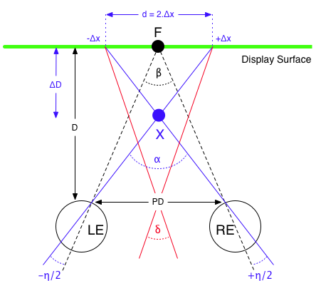
As depicted in the schematic diagram, the spatial shift (Δx) applied relative to the cyclopic projection (x=0) with an opposite sign in each eye (x ± Δx) accounts for the projection on each eye’s retina of a stimulus (X) at some depth (ΔD) relative to a fixation point (F) through these simple geometrical considerations:
![]()
and
![]()
That is:
![]()
Since binocular disparity is given by (see here for more details):
![]()
Substituting ΔD from (1) in (2):
![]()
Noting that:
![]()
One obtains:
![]()
So to specify a binocular disparity of η arcmin (and a depth defined by equation 1), you would apply a spatial shift of ± η/2 arcmin.
In Psykinematix, disparity can be applied to a stimulus as a whole (ie all pixels appear with the same depth) using the “D=” format in the x coordinate or locally using a depth map within the Custom Stimuli.
To present a flat stimulus at a given depth (ie with the same disparity applied to every pixel), you simply indicate a spatial shift to apply to each stimulus version presented to the left and right eyes using the following format for the stimulus x coordinate:
value1; D = value2
where value1 indicates the x coordinate (in deg) of the stimulus and value2 the shift in arc minute (binocular disparity being then 2 x value2).
To present a stimulus with some depth map (each pixel having its own disparity), you have to create 2 versions of the same Custom Stimuli, one for each eye and with opposite sign in their disparity amplitude (± η/2), using the dshiftp() function:
dmax = ... # disparity amplitude in arcmin
disparitymask = dmax*f(x,y,r,theta)
stimulus = g(x,y,r,theta) # carrier
leftimage = dshiftp(stimulus,-disparity)
z = leftimage
dmax = ... # disparity amplitude in arcmin
disparitymask = dmax*f(x,y,r,theta)
stimulus = g(x,y,r,theta) # carrier
z = rightimage
In both cases, the disparity conversion from arcmin to pixel (±Δx) is done automatically with a sub-pixel resolution taking the viewing distance and the display pixel density into account.
✍ If you are not very familiar with stereopsis, we recommend that you experiment with this interactive widget. This widget illustrates graphically the relationship between the parameters that affect stereopsis: drag the blue point X, the green line denoting the display surface, or the slider specifying the pupillary distance (PD).
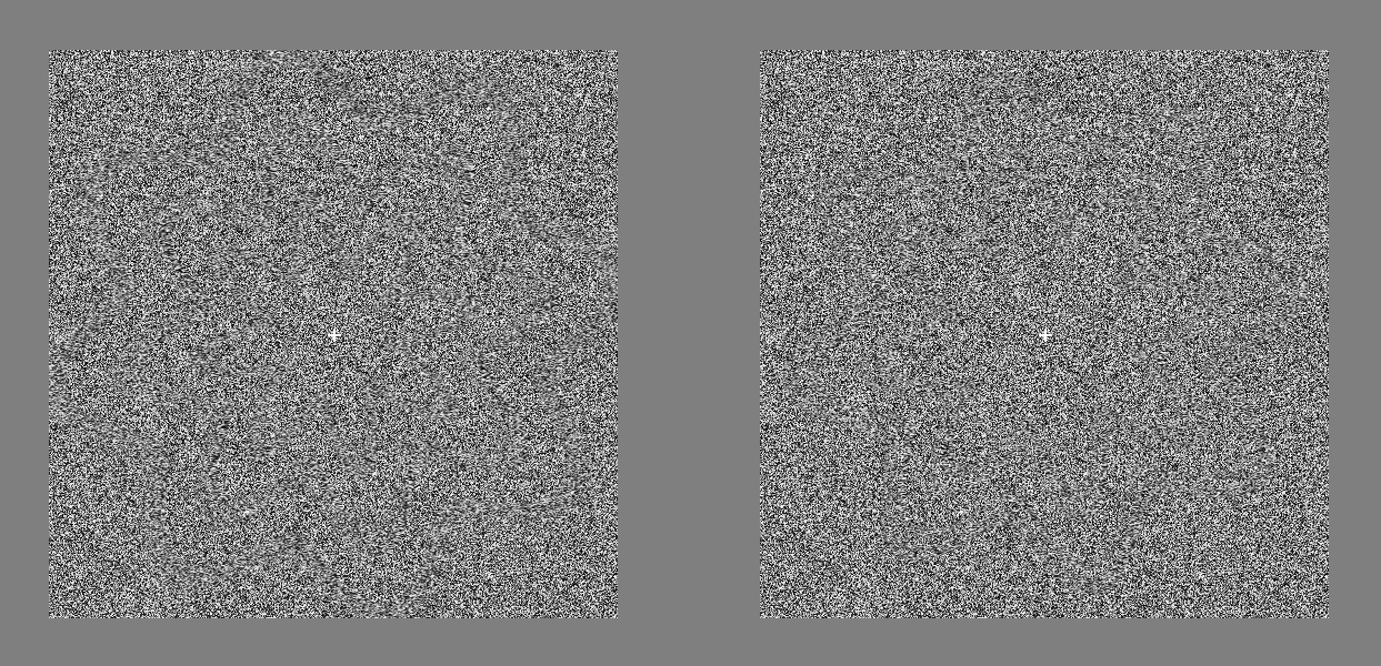
Examples of stereograms created with Psykinematix:
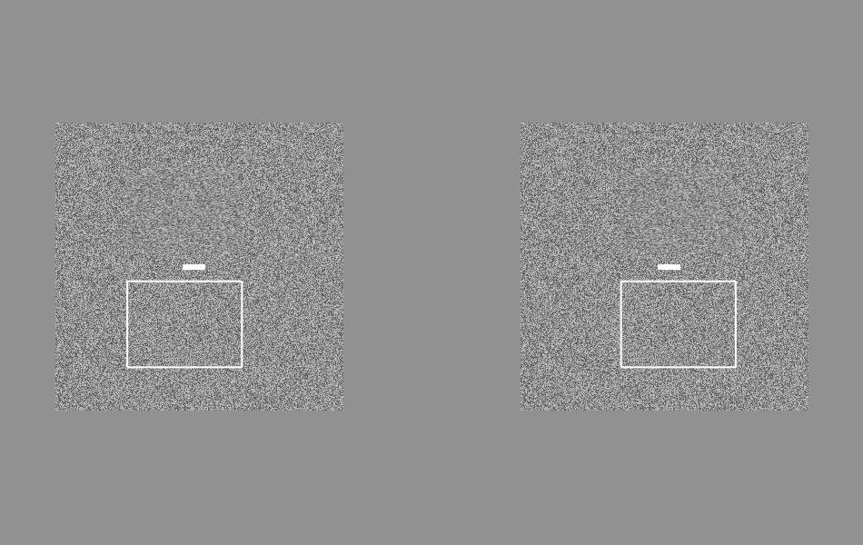
Globally- and locally-defined stereograms created in side-by-side stereo mode which requires crossed-eye free viewing: cross your eyes, so that the pair of images will double to four, and be somewhat out of focus; then slowly uncross your eyes so the 2 central images overlap (tip: use the crosses as an anchor). At some point, the two pairs of images you are seeing will begin to overlap completely and you should perceive the stereogram in the fused central image.
Globally- and locally-defined stereograms for Red-Green Anaglyph glasses.
Using a Cedrus Lumina Controller
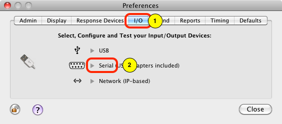
The Lumina controller from Cedrus is a response system designed for use in an fMRI scanner. Here are the steps to follow to make it work reliably with Psykinematix (see also the Preferences and Supported External Devices sections).
First, you will have to set up the Lumina device and test it as illustrated below after connecting it to the computer:
-
Open the Preferences and click on the "I/O" tab,
-
Click on the small arrow next to the Serial option,
-
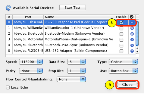
Select in the table the entry corresponding your Lumina device (the one with the port named '/dev/cu.usbserial*'; if there is none then make sure to update the device list by clicking on the small rounded blue arrow in the top-left corner),
-
Set the serial settings for the selected device: Speed of 115200, Parity as None, Data Bits as 8, Stop Bits as 1, Type as Cedrus, Use as Button Box.
-
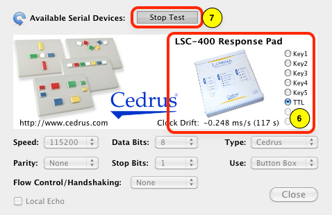
Then click on the "Start Test" button to open the communication with the serial device,
-
If the communication with the serial device is successful, the device table should be replaced by a graphical representation of the device as shown below with an image of the device in use and a list of available buttons/signals (plus a real-time estimate of the device clock drift for timing purpose). If a button is pressed or a TTL triggered, it should show up in the right column (please check all that applies to your setup). Make sure to note the name for each button available on your setup (eg, Key1 for the blue button of the fMRI response pad, Key2 for ... etc).
-
Press the "Stop Test" button to stop the test and return to the device table.
-
If the test was successful, then the cross symbol in the last column should be replaced with a check symbol. Finally make sure to enable the device by checking the "Enable" check box.
-
Click on the "Close" button when you are done with the device testing. The configuration for the device will be saved and automatically retrieved each time the device will be used by your experiment.

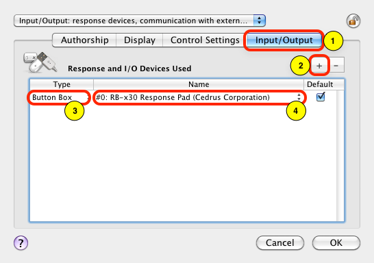
After the device setup, you will have to tell your experiment about using the serial device through its TTL input:
-
Edit the "Input/Output" properties of your mapping experiments (eg the Creating Retinotopic Mapping Stimuli tutorial)
-
Click on the '+' button to add a new device in the table,
-
For the new added device, select Button Box as Type,
-
Select the name of the serial device that has been configured in the I/O Preferences,
-
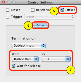
Edit the stimulus properties (eg Annulus Stimulus) and open the Control Settings palette shown below. Check its "Offset" box,
-
Select the "Offset" tab,
-
Specify the termination criterion: it is based on Subject Input using a Button Box with a TTL input. Don't forget to check the "Wait for release" box so the next trial does not start before the TTL goes back to the 0 level.
-
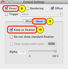
Check the "Onset" box,
-
Select the "Onset" tab,
-
Check the "Keep as fixation" box so the stimulus stays on the screen until the next trial is ready to be presented.
Users have also reported that their Lumina controller was sometimes resetting its mode as soon Psykinematix was trying to communicate with it. In this case, you should manually switch back to the desired mode just after it gets reset. You have about 3 seconds to do so, otherwise Psykinematix would fail communicating with the Lumina controller.
Q: How to present different stimuli simultaneously?
A: Use a Timeline composing and it is easy to specify SOA and ISI between stimuli!
Q: How to randomize a stimulus position at regular intervals?
A: Use an expression like “rnd*2-1::(0.1)” for the stimulus coordinates:
in this example a random value between -1 and 1 is generated every 0.1 second.
You have an unresponded “How To” question? Send it to us and we will try to include it in the next revision of this iBooks: