


With Psykinematix, collected data may be fitted with psychometric functions immediately after each session in addition to fitting automatically performed by a method (Bayesian or of constant stimuli). To access the fitting capabilities, click on the "Plotter" icon in the toolbar to display the Plotter Panel (or press shift–⌘R) and select a graphable data set (last level in the results hierarchy).
Because different data types need to be fitted with different psychometric functions or psychophysical models,
Psykinematix provides custom settings for the following data types:
Performance
Reaction Times
Measurements
The most important customizable option is the fitting function which is constraining
the range (e.g. performance is limited to the 0-100% range)
and shape (e.g. monotonically increasing or decreasing) of the data distribution.
Each available tab provides access to the most
used psychometric functions and psychophysical models associated with each data
type. These tabs can be used to find out what the most appropriate fitting function
is given a data set: simply select the fitting function and some of its properties
to perform a single fit to the data. This provides the best-fit values
for its free parameters (e.g. the alpha and beta parameters for a performance-fitting
psychometric function). However you have to remember than these values are only
estimates that do not take variability in the data into account.... If you want
to know how reliable these free parameter values are in terms of confidence intervals,
standard error, goodness of fit, and stability, you have to use the "Fitting..."
tab which provides those advanced features.
The curving fitting procedure provided by Psykinematix is based on the Levenberg-Marquardt weighted least squares minimization technique (Press et al. 1986). This fitting algorithm can be also associated with a bootstrap analysis, a particular kind of Monte Carlo technique, to estimate the variability of free parameters in the fitting functions or models (Maloney 1990, Foster 1997, Wichmann 2001a, Wichmann 2001b). The bootstrap method is a resampling technique relying on a large number of simulated repetitions of the original experiment. It is well suited to the analysis of psychophysical data because its accuracy does not rely on large numbers of trials as do methods derived from asymptotic theory (like the probit analysis).
In short, the weighted least-squares fitting procedure minimizes the sum of the square of the errors between the n measured data points (datai) and the corresponding model predictions (modeli) weighted by some factor (weighti), expressed as:
![]()
The weights can take different forms (see Weighting
scheme option below). ![]() (Chi-Square) is also used to specified
the goodness of the fit.
(Chi-Square) is also used to specified
the goodness of the fit.

Fitting methods:
- Standard: The standard procedure fits the original data with random initial
values for the free parameters, reports
the best-fit parameter values without providing any precision, and optionally
checks the stability of the solution. To obtain an estimate of the variability
of the free parameters, a bootstrap analysis is required:
- Nonparametric bootstrap: many data sets are generated by adding noise to
the original data set (the amount of noise depends on the know variability
of the original data) and each of them is fitted
with the same function. Statistics of the free parameters are then
derived from the distribution of the best-fit parameter values.
- Parametric bootstrap: many data sets are generated by adding noise to the fit performed on the original data set (the amount of noise depends on the Root Mean Squared Error, RMSE, of the original fit) and each of them is fitted with the same function. Statistics of the free parameters are then derived from the distribution of the best-fit parameter values.
Note that the nonparametric bootstrap uses the measurements to generate the simulaled datasets, while the parametric bootstrap uses the model responses for the simulated data sets. The choice between nonparametric and parametric bootstrap analysis depends then on how much confidence you have in the measured data as against the confidence you have about the underlying mechanism that gives rise to the measured data.
Weighting scheme:
- None: the least squares fitting is often done by simply minimizing
the sum-of-squares of the vertical distances of the data from the function
values, i.e. without weighting (weighti =
1 for all data points). However in many experimental conditions, the average
absolute value of these distances of the points from the curve is higher when
the data point has a higher value, i.e. the standard deviation of the error
is not consistent along the graph, and some weighting is required to
reflect this variability and better balance the influence of each data point.
Several weighting options are available:
- Standard deviation: this weighting is appropriate when the variance
of the measurement error is known. Note that this weighting scheme is not
always the best choice if a small number of measurements have been collected
because the standard deviation may then considerably vary just by
chance. The relative and Poisson weighting schemes are sometimes more appropriate
in these cases.
- Relative weighting: this weighting is appropriate if
you want all the points to have about equal influence on the goodness-of-fit.
- Poisson weighting: this weighting is appropriate if you want a compromise between minimizing the absolute distance squared and minimizing the relative distance square, or if you know that the values follow a Poisson distribution (i.e. standard deviation being approximately equal to the square root of the mean).
Goodness of fit:
-
R2 (coefficient of determination): This statistic measures how successful the fit is in explaining the variation of the data. Put another way, R2 is the square of the correlation between the response values and the predicted response values. It is also called the square of the multiple correlation coefficient and the coefficient of multiple determination. R2 can take on any value between 0 and 1, with a value closer to 1 indicating that a greater proportion of variance is accounted for by the model. For example, an R2 value of 0.8 means that the fit explains 80% of the total variation in the data about the average.
- RMSE (Root Mean Squared Error): This statistic
is also known as the fit standard error and the standard error of the regression.
It is also an estimate of the standard deviation of the random component in
the data, and is defined as the square-root of the mean square error or the
residual mean square (the residual sum of squares divided by the degrees of
freedom df defined as the number of response values n minus
the number of fitted coefficients m estimated from the response values).
Just as with
 ,
an RMSE value closer to 0 indicates a fit that is more useful for prediction.
Note that the RMSE returned by Psykinematix is an unweighted version (see the
reduced Chi-Squared below for a weighted version).
,
an RMSE value closer to 0 indicates a fit that is more useful for prediction.
Note that the RMSE returned by Psykinematix is an unweighted version (see the
reduced Chi-Squared below for a weighted version).
-
 (reduced
Chi-Squared): The reduced chi-squared statistic is simply the chi-squared
divided by the number of degrees of freedom df. A rule of
thumb is that a “typical” value
of for
a “moderately” good
fit is χ2 ≈ df, that is ≈ 1
which indicates that the extent of the match between observations and estimates
is in accord with the error variance. A large indicates
a poor model fit. However < 1
indicates that the model is 'over-fitting' the data (either the model is
improperly fitting noise, or the error variance has been over-estimated).
A > 1
indicates that the fit has not fully captured the data (or that the error
variance has been under-estimated).
(reduced
Chi-Squared): The reduced chi-squared statistic is simply the chi-squared
divided by the number of degrees of freedom df. A rule of
thumb is that a “typical” value
of for
a “moderately” good
fit is χ2 ≈ df, that is ≈ 1
which indicates that the extent of the match between observations and estimates
is in accord with the error variance. A large indicates
a poor model fit. However < 1
indicates that the model is 'over-fitting' the data (either the model is
improperly fitting noise, or the error variance has been over-estimated).
A > 1
indicates that the fit has not fully captured the data (or that the error
variance has been under-estimated).
-
Q: The Q measure is a distribution
function that gives the probability that the minimum is as
large as it is purely by chance. For small Q values, the deviation
from the model is unlikely to be due to chance and the model may be incorrect.
For larger Q values,
the deviation from the model is more likely to arise by chance suggesting the
model is an adequate description of the data. A Q of 0.1 suggests
an acceptable model fit. If Q is larger than, say, 0.1, then
the goodness-of-fit is believable. If it is larger than, say, 0.001, then the
fit may be acceptable if the errors are nonnormal or have been moderately underestimated.
If Q is less than 0.001 then the model and/or estimation procedure
can rightly be called into question (Press et al. 1986).
At the opposite extreme, it sometimes happens that the probability Q
is too large, too near to 1, literally too good to be true!
Free Parameter Precision:
-
Standard Errors: the standard deviation of the best-fit parameter values obtained through the bootstrap analysis.
- 95% CIs: the 95% confidence intervals obtained through
the bootstrap analysis, i.e. mean ± std * t(95%, df).
- 99% CIs: the 99% confidence intervals obtained through the bootstrap analysis, i.e. mean ± std * t(99%, df).
Check stability: because the fitting procedure with the specified psychometric function or model may be sensitive to starting values of the free parameters, it may be necessary to verify the stability of the fits. This is performed by adding noise to the free parameters and refitting to the data. The fitting procedure is considered as stable when the refitting provide values that match the free parameters statistics. Unstable parameters are followed by the * symbol in the plotted graph.
Nb samples: the number of iterations for finding the initial best-fit parameters, running the bootstrapping procedure and checking the stability.
Start/Stop: this button launches or stops the computer-intensive fitting procedure running in a separate thread so it does not interfer with the normal functions of Psykinematix. Note that the progress of the fitting procedure is reflected with a progress indicator in the Plotter panel and in the toolbar.
Remember that nonlinear curve fitting is no
magic: a successful fit is highly dependent on the quality of the measured
data, the selection of an appropriate function and a reasonable degrees
of freedom.
We recommend you to take a look at this free book available online (Motulsky
2003)
as this section cannot cover the complex methodology of nonlinear
fitting.
Fitting Psychometric Functions to Performance Data
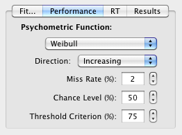
Subject's performance (% correct) as a function of some stimuli parameters (dependent variable) can be freely fitted from the "Performance" tab: the psychometric function, its direction (the relationship between performance and the dependent variable is assumed to be monotonic, either increasing or decreasing), miss rate, chance level and threshold criterion should be chosen appropriately to reflect the experimental constraints (eg: a chance level of 50% in a 2AFC).
All the available psychometric functions are cumulative distribution function (CDF) types of the form:
for a monotonic increase |
|
 |
for a monotonic decrease |
where ![]() is the performance as a function of some stimulus parameter
is the performance as a function of some stimulus parameter ![]() ,
,
![]() is the chance level (eg: 50% in a 2AFC),
is the chance level (eg: 50% in a 2AFC),
![]() is the miss rate,
is the miss rate,
![]() is
the cumulative distribution function, with
is
the cumulative distribution function, with ![]() being
the stimulus parameter,
being
the stimulus parameter, ![]() and
and ![]() are
the sensitivity parameters that control the shape of the function. The available
psychometric functions are the ones typically used in visual psychophysics and
can be also used as models for the Method
of Constant Stimuli or
the Bayesian Method:
are
the sensitivity parameters that control the shape of the function. The available
psychometric functions are the ones typically used in visual psychophysics and
can be also used as models for the Method
of Constant Stimuli or
the Bayesian Method:
| Weibull CDF | |
| Logistic CDF | |
| Right Gumbel CDF | |
| Right Gumbel CDF | |
| Left Gumbel CDF |
Note that for the Weibull function, ![]() and
and ![]() are
analogous (but not similar!) to the threshold and slope respectively, while
for all other functions they are analogous to the offset and spread respectively.
The threshold (t) and slope (s)
for a specified probability level (p) (threshold criterion) of the
psychometric functions are defined as:
are
analogous (but not similar!) to the threshold and slope respectively, while
for all other functions they are analogous to the offset and spread respectively.
The threshold (t) and slope (s)
for a specified probability level (p) (threshold criterion) of the
psychometric functions are defined as:
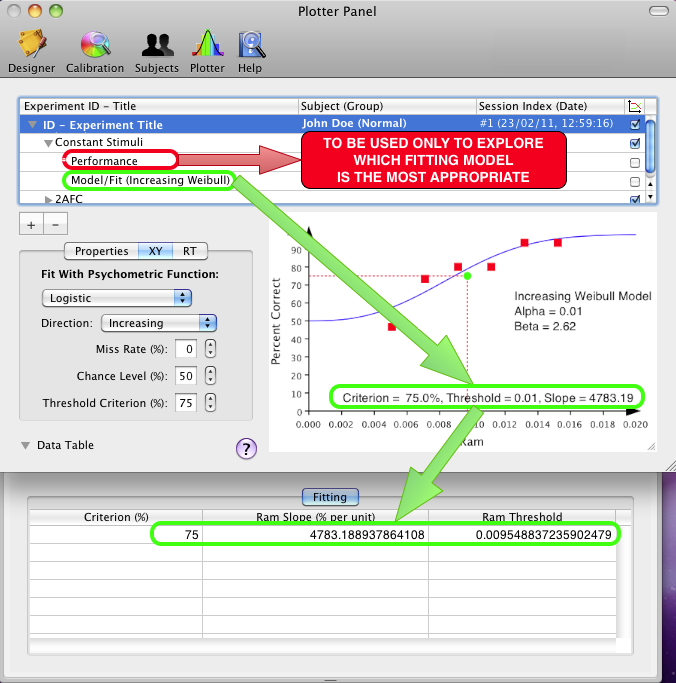
A typical scenario is illustrated below where a method provides 2 graphable data sets: a "Performance" set that plots % correct as function of the dependent variable, which can be freely fitted, and a "Model/Fit" set that plots the same data but pre-fitted with the psychometric function that was indicated under the Method Panel (the resulting fitted parameters are those shown under the "Fitting" tab in the data table associated to the 1st level of the session results). The "Model/Fit" fitting cannot be modified, and the fitting of the "Performance" set should be used at the pilot stage to discover the most appropriate psychometric function or when the pre-specified function does not properly fit a specific data set.
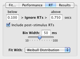
The distribution of reaction times collected in a procedure can be plotted and fitted from the "RT" tab. The graphical representation of the reaction times can be customized: reaction times below a given level (anticipatory responses) and above a given level (late responses) can be filtered out, and the bin width can be set to any value between 10 and 100 ms. Post-stimulus RTs are included by default, but can be excluded from the histogram representation by unchecking the related check box.
The reaction time distribution can be fitted with a Weibull distribution using its probability density function:

where k > 0 is the shape parameter, λ > 0 is the scale parameter of the distribution, and ![]() is a translation parameter.
is a translation parameter.
The mean and standard deviation of the Weibull distribution are given by:
![]()
![]()
Note that the accuracy of the fitting procedure depends on the bin width.
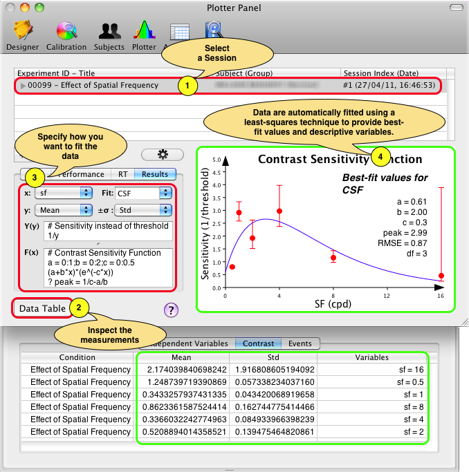
Fitting Models to Measurements
The "Results" tab gives access to custom fitting of experimental measurements such as thresholds and slopes as function of some independent variables or conditions. These measurements are generally associated with summary data presented at the 1st level of the session results (e.g. "Contrast" tab). A typical example is contrast thresholds measured as function of spatial frequency (obtained through a method of constant stimuli or a staircase) which can then be fitted with a contrast sensitivity function (this example is illlustrated in the Contrast Sensitivity Task Tutorial: Effect of spatial frequency).
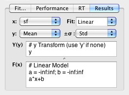
To perform a custom fit you simply need to specify the x and y data to be fitted, the fitting function and optionally the standard deviation of the y data. You can add your own fitting functions but some popular ones are already included: linear regression, contrast sensitivity function (CSF), variance summation model (VSM) and dipper function (TvC).
Each fitting function consists in the specification of Y(y), an optional y-transform in case the y data needs to be plotted differently than they have been collected (e.g. plotted as sensitivities instead of thresholds), and F(x) the function to be fitted to Y(y). If no y-transform is required, then simply specify 'y' for Y(y). The fitting function can be any arbitrary expression where:
- the # symbol is used to provide comments,
- the free parameters and their valid ranges are defined by the format: 'var
= minimum value : maximum value',
- the last value without assignment is the value returned by the function ('a*x+b' in the above example),
- output variables are defined by the format '? var = expression'. Output variables should be descriptive properties of the model derived from the best-fit values of the free parameters (e.g. the peak frequency of the CSF).
To add a new function or modify a pre-existing one, select the 'Add New' option in the Fit pop-up menu to duplicate the previous selection and then change its name and definition. Select 'Remove' to delete the currently selected function (note that only user-defined functions can be modified or deleted). User-defined fitting functions are automatically saved in Psykinematix preferences.
Foster, D. H., & Bischof, W. F. (1997) Bootstrap estimates of the statistical accuracy of thresholds obtained from psychometric functions. Spatial Vision, 11(1), 135-139 (PDF)
Klein, S. A. (2001) Measuring, estimating, and understanding the psychometric function: A commentary. Perception & Psychophysics, 63 (8), 1421-1455 (PDF)
Maloney, L. T. (1990) Confidence intervals for the parameters of psychometric functions. Attention, Perception, & Psychophysics, 47(2), 127-134 (PDF)
Motulsky, H., & Christopoulos, A. (2003) Fitting Models to Biological Data Using Linear and Nonlinear Regression: A Practical Guide to Curve Fitting. 2003, GraphPad Software Inc., San Diego CA, graphpad.com. (PDF)
Press, W .H., Flannery, B. P., Teukolsky, S. A., & Vetterling, V. T. (1986) Numerical Recipes. Cambridge University Press (HTML Link)
Wichmann, F. A. & Hill, N. J. (2001a) The psychometric function: I. Fitting, sampling and goodness-of-fit. Perception and Psychophysics 63(8), 1293-1313 (PDF)
Wichmann, F. A. & Hill, N. J. (2001b) The psychometric function: II. Bootstrap-based confidence intervals and sampling. Perception and Psychophysics 63(8), 1314-1329 (PDF)